Excel Basics: 6 Formatting Techniques That Will Dramatically Improve the Appearance of Your Spreadsheets

A little formatting goes a long way when it comes to improving the appearance of your Excel spreadsheets.
Beyond making your Excel workbooks look more professional, consistent formatting will help spreadsheet users better understand your data and the purpose of each section. A well-designed, thoughtfully formatted spreadsheet is sure to impress your colleagues.
None of the formatting techniques outlined in this article are difficult to apply but they’ll make a big difference to your spreadsheets!
Here are 6 formatting techniques that will elevate the appearance of your spreadsheets, along with the steps I took to format the included sample worksheet.
1) Use a Larger Font for Main Titles
The main title in your spreadsheet should be bigger than your headings and numbers.
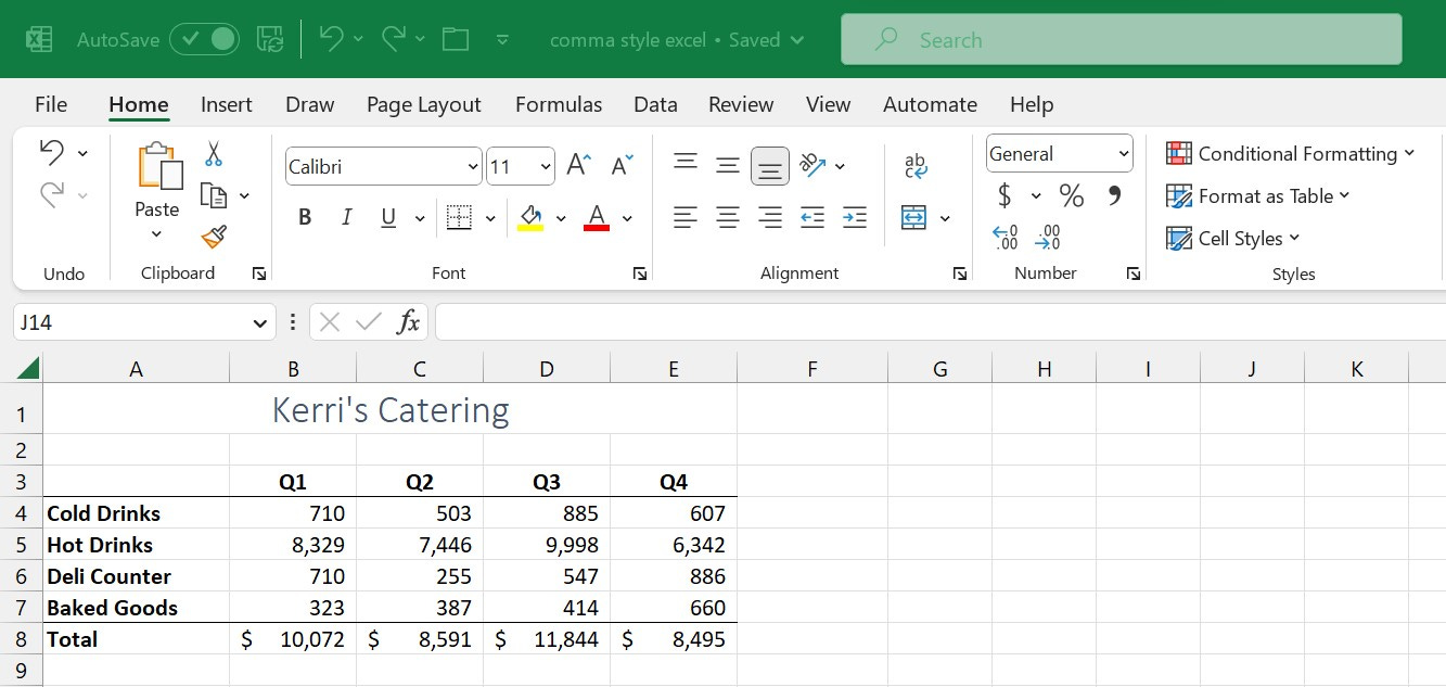
In the spreadsheet below, I applied the Title style to Kerri’s Catering then I centered it above my worksheet.
Excel includes dozens of predefined styles.
I clicked the Cell Styles button in the Home > Styles group and selected Title from the gallery’s Titles and Headings section. Next, I dragged to select A1:E1 and clicked the Merge & Center button in the Home > Alignment group.
2) Make Headings Bold
Headings should clearly identify the purpose of each row and column in your worksheet.
I dragged to select the category headings in A4:A8 then I clicked the Bold button in the Home > Font group. Next, I selected B3:E3 and applied bold formatting to the fiscal quarters before clicking Center in the Home > Alignment group.
3) Use Comma Style for Detailed Revenue Numbers
I advocate using Comma Style for detailed revenue numbers. People will understand that these values represent dollar amounts but you don’t need to add clutter to your worksheet by including the currency symbol. You can further simplify your spreadsheet by eliminating decimal places when referencing whole numbers.
I dragged to select B4:E7 then clicked the Cell Styles button in the Home > Styles group before selecting Comma [0] from the gallery’s Number Format section.
4) Use Accounting Number Format for Subtotals and Totals
I recommend displaying a currency symbol for subtotals and totals so it’s obvious that your spreadsheet includes dollar amounts.
After selecting B8:E8, I clicked the Cell Styles button in the Home > Styles group then chose Currency [0] from the gallery’s Number Format section. Currency [0] adds the dollar sign and eliminates the decimal places.
5) Add Borders to Separate the Sections
I like to visually separate headings and totals from the detailed revenue numbers.
I dragged to select A3:E3 then clicked the down-arrow next to the Border button in the Home > Font group and selected Bottom Border from the gallery. I repeated the process for A7:E7.
6) Adjust Column Widths as Necessary
Excel worksheets always look better if you adjust column widths to provide adequate space.
In the sample worksheet above, I positioned my pointer on the border between the headings for column A and B then I dragged to set the width of column A to 15 characters. Next, I dragged across each of the headings for columns B through E before right-clicking in the highlighted area and selecting Column Width from the shortcut menu. I typed 10 in the Column Width box and clicked OK.
What’s Next?
The ability to format worksheets is one of the basic skills every Excel user should have.
Formatting your worksheets consistently will give them a professional appearance and make them much easier to interpret.
Next: Using Formulas to Perform Calculations and Analyze Data


